This is the second installment of a three part series. If you haven’t read part one, check it out HERE
I'd really love it if you would help
spread my message through social media.

As a big THANKS you can download my
Exclusive Excel Shortcut Cheat Sheet

 Click here to Download
Practical Excel Hacks that will save you time, headaches, and hair pulling
Turn positive numbers into negatives with paste special
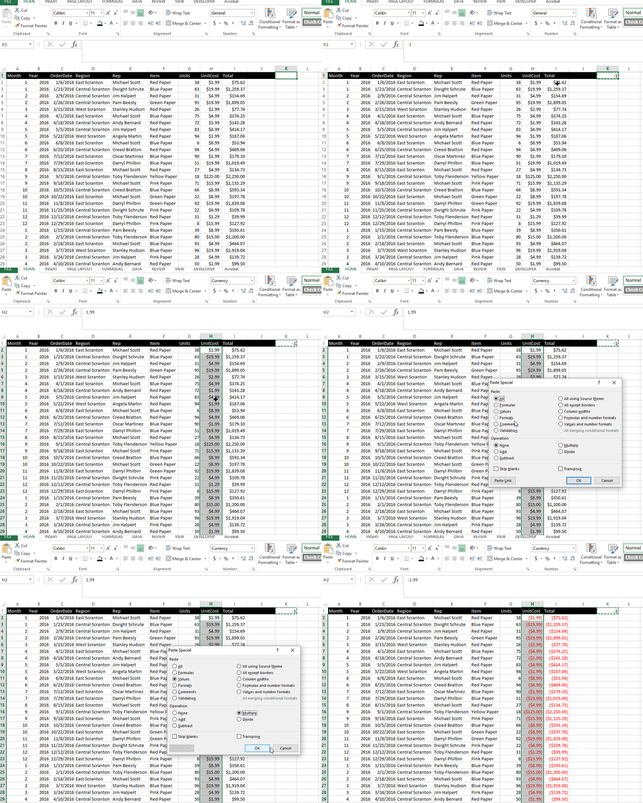
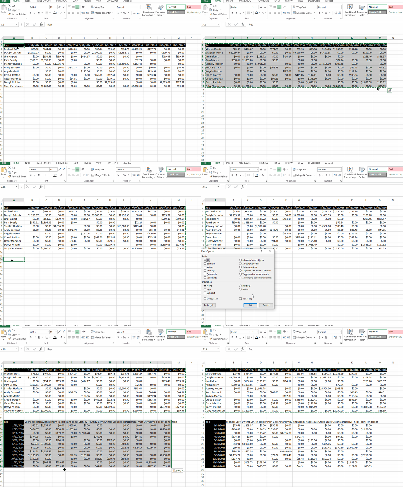
You have a list of numbers and need to reverse the signs? Enter -1 into a cell and use paste special.
Once you have a cell containing -1, copy that cell, select the numbers you want to reverse the signs for and copy, right click and select “Paste Special” (or Ctrl + Alt + V).
Once you have the window open, select values, then multiply, and hit ok.
Use paste special to transpose a table
Have a table or a list and you need to transpose the rows into columns (or columns into rows)? Paste special can also help with that.
Use numbering system to help make VLOOKUPS easier
You love using VLOOKUPS (who doesn’t, right?!) but hate counting columns. Easy fix, just add column numbers along the top of your table to make it easier on you to reference.
Become a formula NINJA with named ranges!
Named ranges are to an Excel user what a lightsaber is to a Jedi knight. You can continue struggling to enter formulas and later deciphering what your formulas do, or you can use named ranges and make your life easier.
When you name a range you’re giving meaning to an otherwise meaningless Excel range. A1:C25 turns into hourly_rate and all of a sudden your formula doesn’t look like Japanese.
You can write “hourly_rate” inside your formula and excel automatically knows exactly where to go to find its data
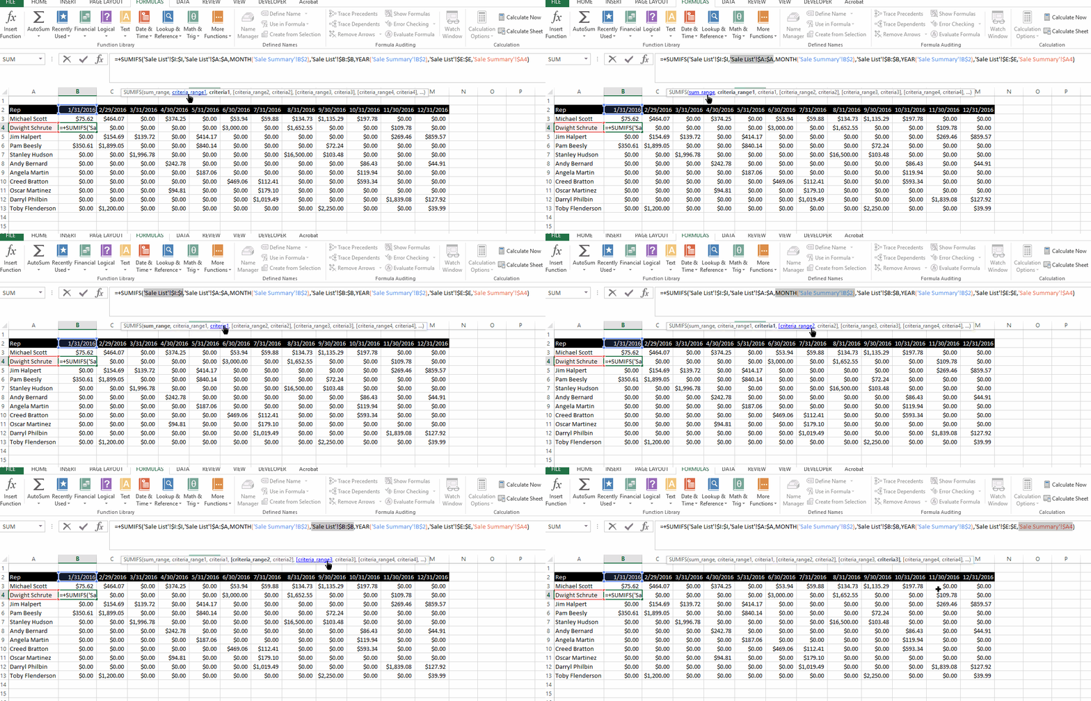
Select arguments via formula tip window
You can make it easier on yourself to enter formula arguments by selecting them inside the formula tip window. Better yet, you can make it easier on yourself to audit your formulas with this little trick.
Break complicated formulas into smaller pieces
Sure, it’s impressive to others when they see your work and Instead of trying to write a complicated formula in one cell, break it out into pieces in separate cells. Make sure each piece works as intended and make sure you ensue each piece is labeled and descriptive to a new user.
This does three things, it makes it easier on you to explain your sheet to others, makes it easier for you to understand how to replicate and update your sheet when necessary, and when bugs arise it is easy to figure out which step in the chain is broken.
Easy, peasy!
You can always combine the individual pieces and impress everyone
Still want to impress everyone by having extra long, complicated formulas? No problem, just follow the last tip, select the necessary arguments using the formula tip window, and just copy and paste!
Use custom formatting to create descriptive labels
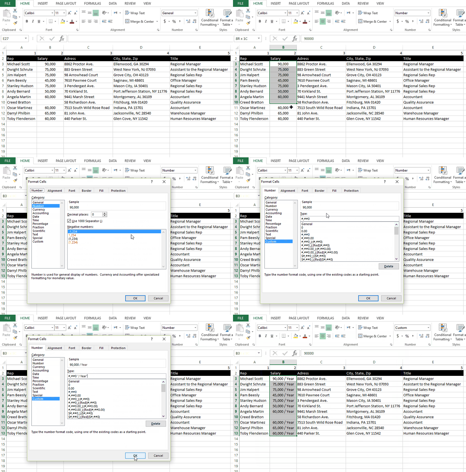
Numbers mean nothing without context, but excel lets you add that context right into your cells without compromising the cell’s data. You can use custom formatting to make numbers and labels more descriptive.
This works with dates as well.
Use concatenate, or ‘&’, to merge text values
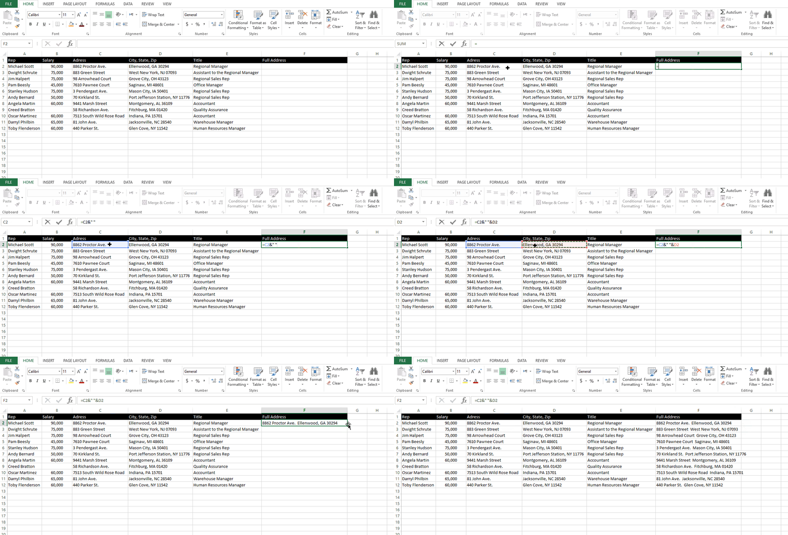
You can merge text strings from different cells into one by using concatenate, or “&”.
If you’re wondering how this seemingly minimal trick can be used in a practical scenario…
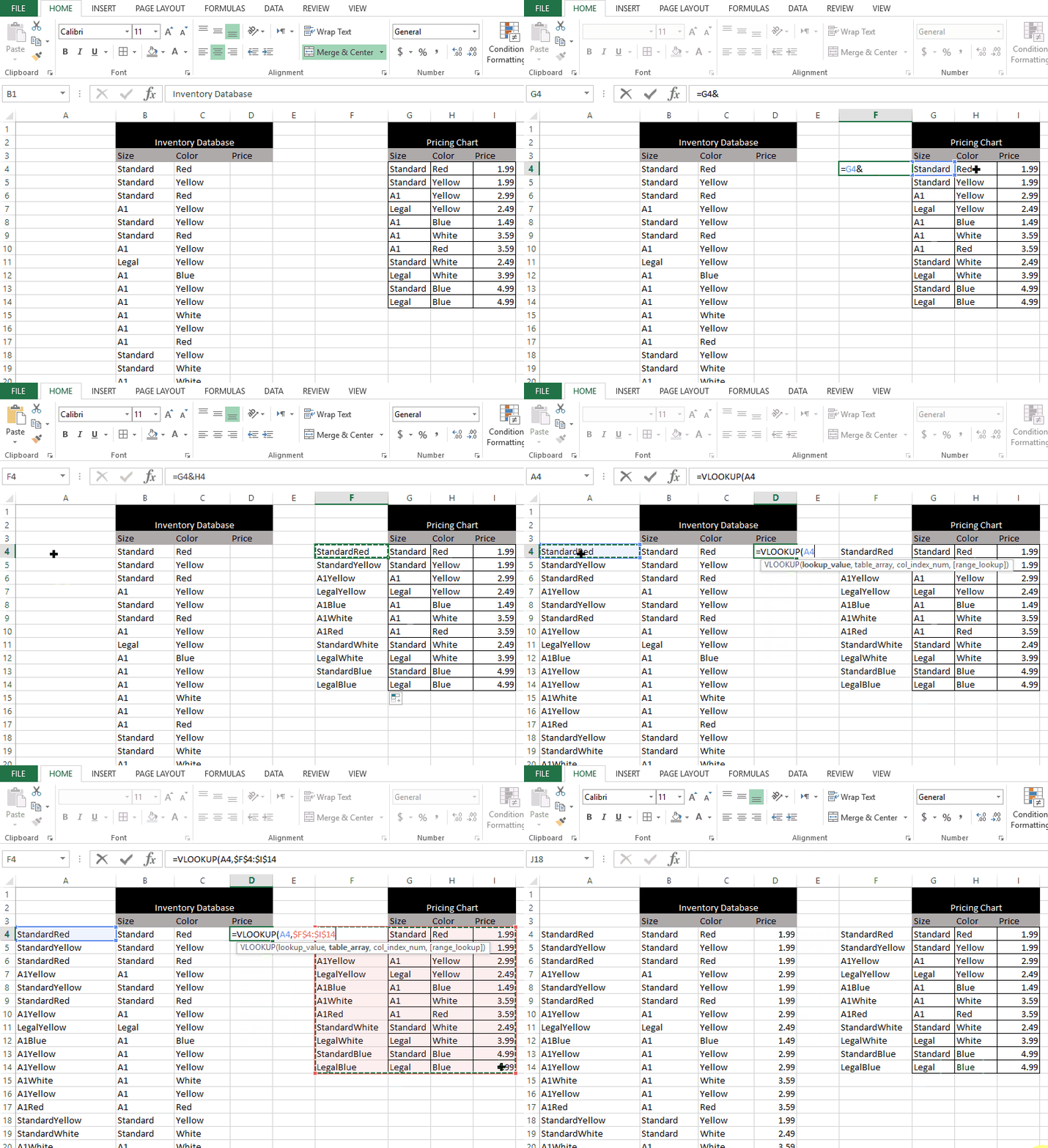
VLOOKUP with multiple lookup criteria.
One of VLOOKUP’s many limitations is that you can only use one criteria to lookup data in another table. But, concatenating text strings allows you to create a unique index and perform VLOOKUPS with multiple criteria.
Make changes to multiple tabs at once
If you select multiple tabs while holding CTRL and enter something into a cell on one tab, this value gets entered in the exact cell on all tabs you have selected.
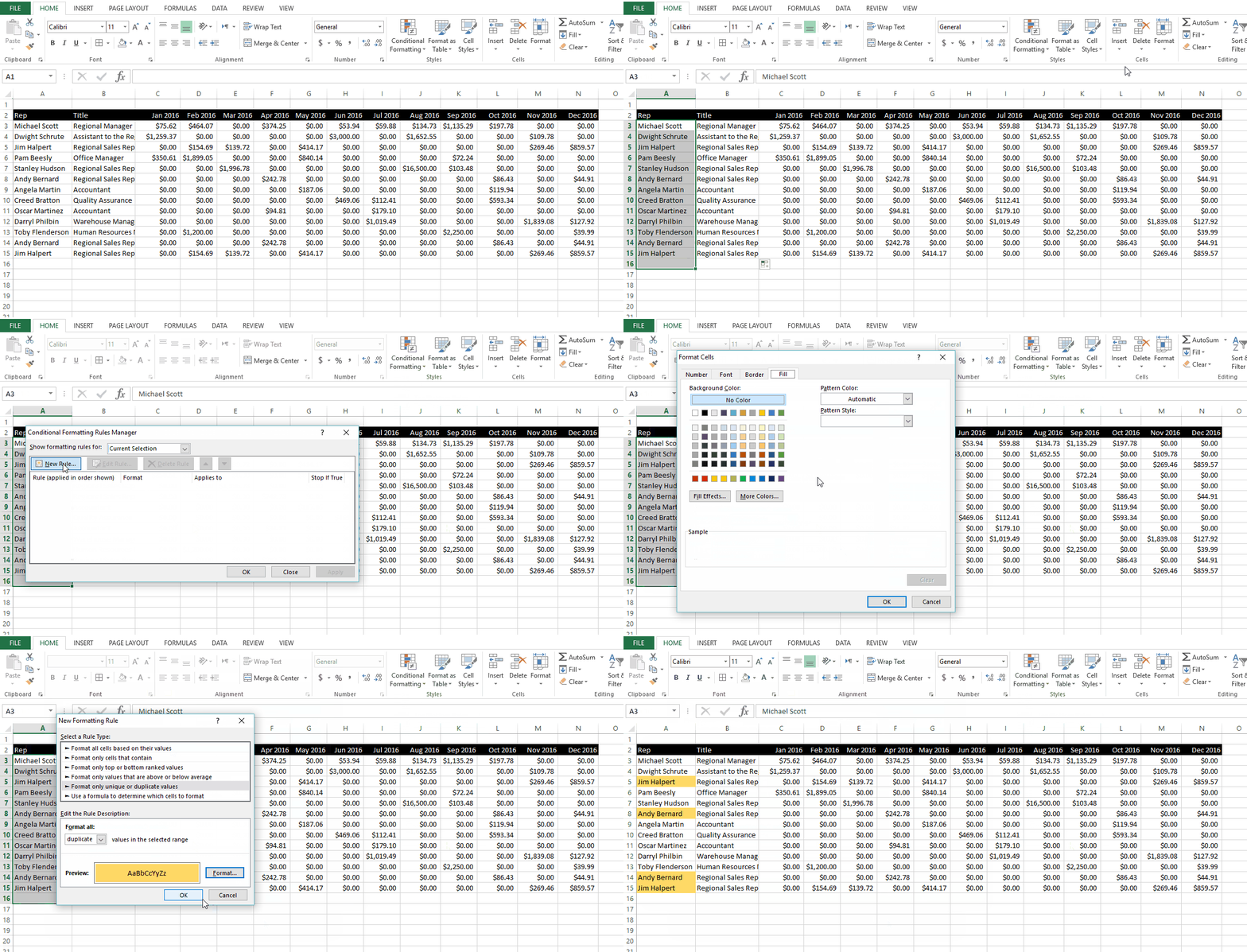
Spot duplicates
If you have a long list of values and you want to see if you have any duplicates, you can easily use conditional formatting to highlight any duplicates, then use your filters to display those values.
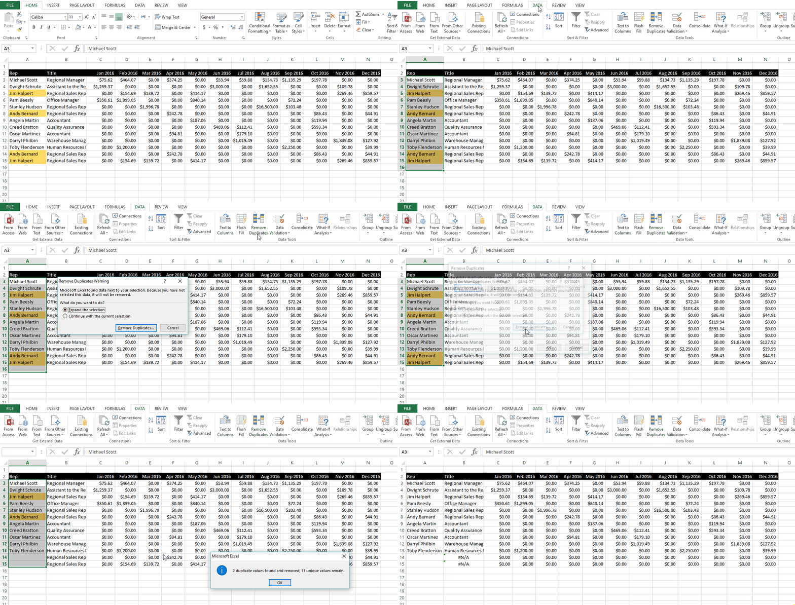
Remove Duplicates
Building on the last tip, you can also automatically remove duplicate values in your sheet by using Excel’s “Remove Duplicates” tool.
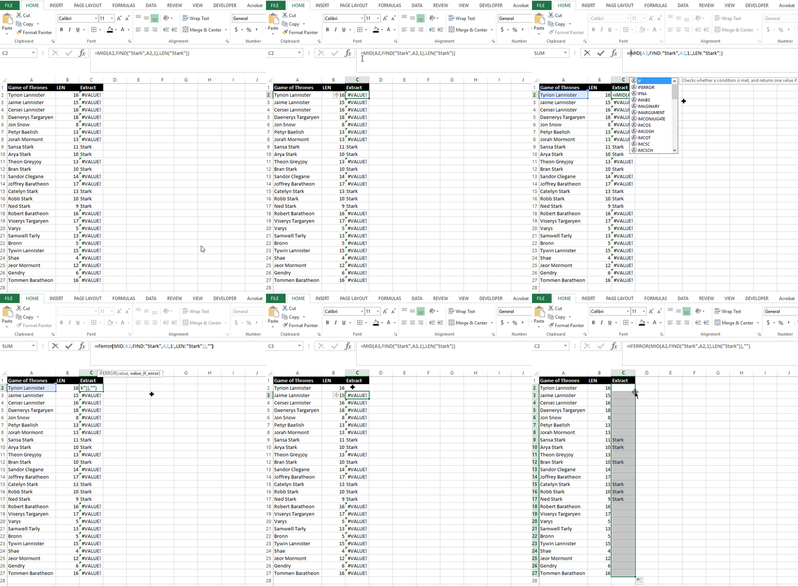
Extract specific text within a cell
=mid([cell extracting from],find([text],[cell extracting from],1),len([text]))
FIND – Finds the text within the text string and returns which character that text string begins. For example, the word “Stark” begins in character number 7 within the text string “Sansa Stark”.
LEN – Returns the number of characters in the word “Stark” (5).
MID – Uses the number 7 returned by FIND and begins extracting characters at this point in the text string. Since LEN returned the number 5, the formula knows to only extract 5 characters to get the word “Stark” from the string “Sansa Stark”.
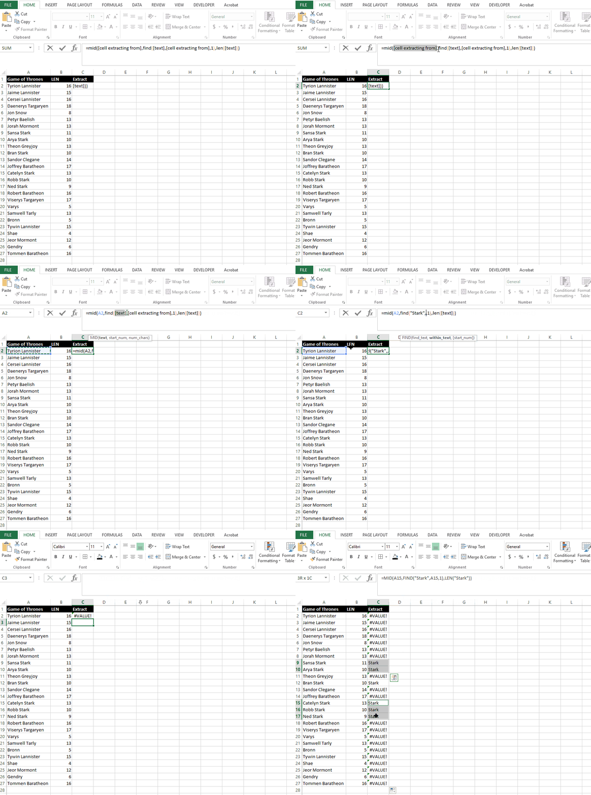
If you want to eliminate the errors when excel doesn’t find what you’re looking for, wrap it in an IFERROR
=IFERROR(mid([cell extracting from],find([text],[cell extracting from],1),len([text])),”Not Found”)
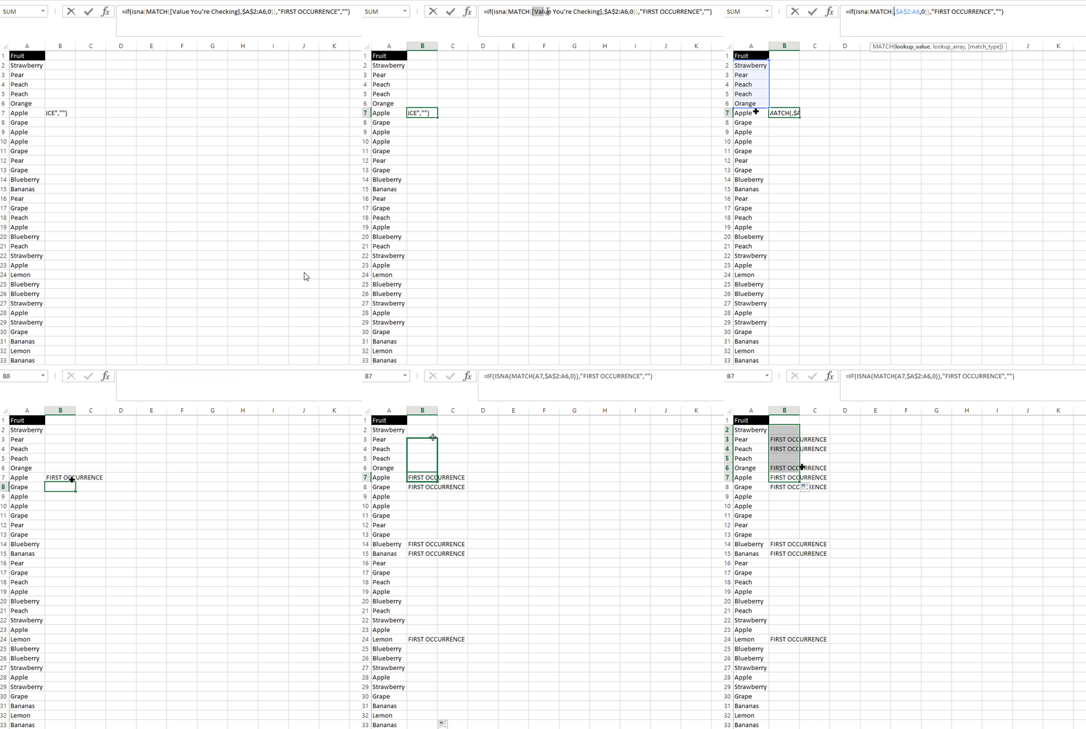
Check if it is a first occurrence within a list of values
This trick is handy whenever you need to figure out which values are unique in a list.
=if(isna(MATCH([Value You’re Checking],[List, ie. $A$2:A6],0)),”FIRST OCCURRENCE”,””)
MATCH – Checks whether the value you’re evaluating is a first occurrence in the list by searching for this value within the list before it. As the formula is copied down the range expands thanks to the combination of absolute and relative cell references (ie. $A$2 stays fixed while A6 shifts to A7, A8, and so on). The MATCH function returns an #N/A error when it is a first occurrence.
ISNA – Evaluates whether the result of MATCH is an #N/A error or not. If it is (which means it’s a first occurrence, it returns a TRUE ir FALSE.
IF – Takes the TRUE or FALSE returned by ISNA and returns the text string “FIRST OCCURRENCE” when its true and blank (indicated by entering “”) if its is FALSE.
Calculate the business days between two dates
NETWORKDAYS calculates approximately how many business days there are between two dates.
=NETWORKDAYS([Start date],[End date])
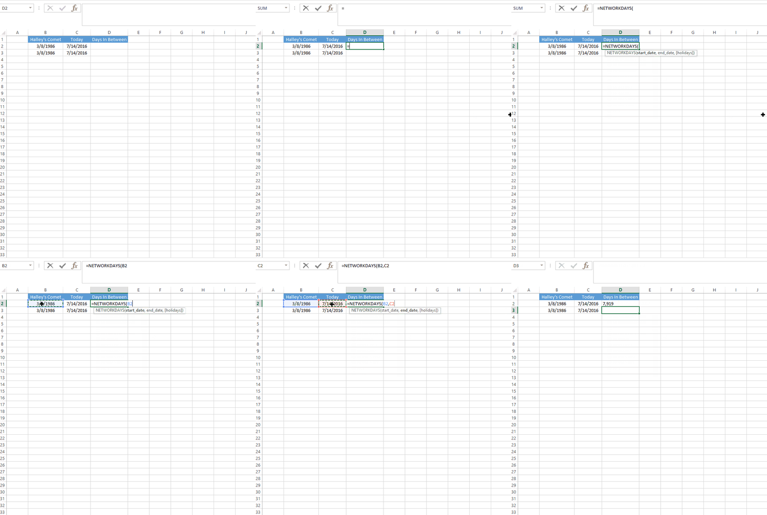
There have been approximately 7,915 business days since Halley’s comet visited earth (at the time of this writing 🙂 )
Get exact number of months, years between two dates
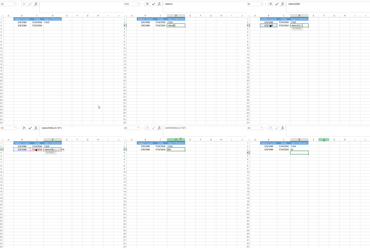
DATEFID gives you the amount of time between two dates represented by month, days, or years depending on what you specify.
Please note that this function is a secret Excel function. Reason is because it’s not listed anywhere and when you try and use it Excel will offer no help for it. Instead, you need to memorize the syntax and use it like a pro despite the lack of help 🙂
=DATEDIF([Start date],[End date], unit)
In this function, unit is a string abbreviation of the unit of time (ie. “M” = month, “Y” = year).
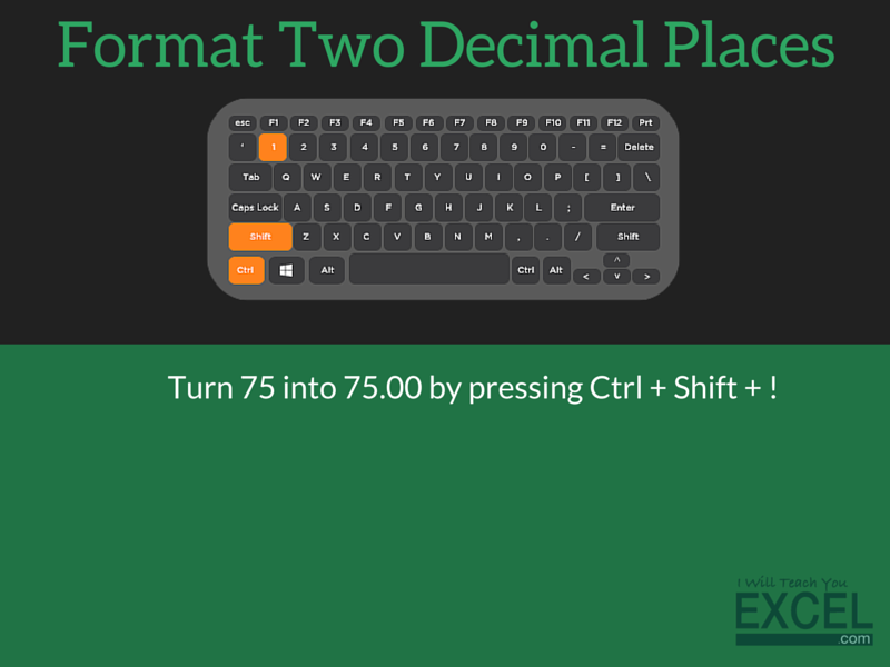
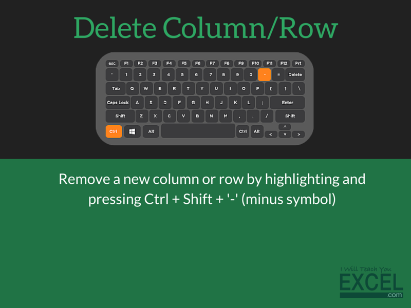
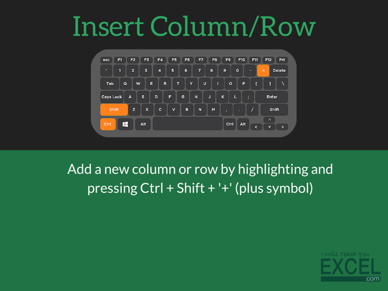
Useful Excel Shortcuts that will save you time
With keyboard shortcuts, focus on creating habits to that lead to muscle memory instead of mental memory. If you’ve played sports before you know what I mean; a baseball player doesn’t think about whether they are turning their hips during a swing, they just do it.
This works the same way. Your goal is to get to the point where your fingers just move directly to the keys that activate the intended action in Excel without you having to give it much thought. There are plenty of shortcuts that I use every day, but if you ask me to tell you which keys I press I’d give you a blank stare.
I'd really love it if you would help
spread my message through social media.

As a big THANKS you can download my
Exclusive Excel Shortcut Cheat Sheet

 Click here to Download

