Ever have a cell that contains a value and you wished you can go in and extract a small piece of the value but leave the rest behind (ie. just the last name in a list of names)? How do you go about doing so? Well, you can go one by one and do it manually or ask one of your co-workers. You could also just use one of the functions we’re about to discuss.
How it works
LEFT, RIGHT, and MID are functions used to extract alphanumeric characters from other cells. Lets say you have a cell that contains the text “Invoice 123456” and you just need the invoice numbers for a VLOOKUP; use the RIGHT function to get those numbers. Here is an example:
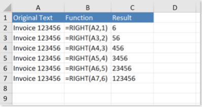
As you can see, the RIGHT function begins on the right side of the cell, and extracts exactly how many characters you tell it to by moving in sequential order towards the left side. LEFT does the same thing, except you begin from the left side instead of the right.
The Syntax
Here is how the syntax works for both LEFT and RIGHT
=RIGHT(Text, Number of Characters)
=LEFT(Text, Number of Characters)
Text – This is the value or cell containing the characters you want to extract.
Number of Characters – The number of characters you want to extract.
The MID Function
Pretty straight forward, right? Now, lets talk about MID. MID does the same thing that LEFT and RIGHT do, except it starts extracting from any point within the string of characters (not just exclusively from the left or right side). Take a look at the text string below:
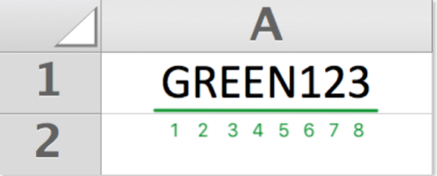
What do I do if I need to extract the middle four characters (“EEN1”) from this text string?
I can accomplish this using MID because it not only asks for how many characters you want to extract, but also asks where you want to begin extracting from. In our case, I want to extract the characters “EEN1” so I would need to tell the function to begin from the 3rd character in the string (the first “E”).
Here is what it would look like:
MID(text, start number, number of characters)
=MID(A1,3,4)=EEN1
Text – This is the value or cell containing the characters you want to extract.
Start Number – This is where MID makes all the difference. Here, you tell it which character number to begin from. In our example, we chose the number 3 because we needed it to start at the first “E”.
Number of Characters – The number of characters you want to extract.
Lets look at some more examples:
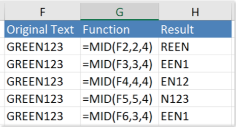
As you can see, the only thing that changes in our example is which character within the string of characters we’re starting from.
The FIND + MID functions
There is a bonus text function that few excel users know about. If you were looking for a specific set of characters within another string (ie. Anyone with “Joel” in their name in a list of names), you could use the FIND function. FIND, as the name implies, helps you find any set of characters within another set of characters.
Here is how it works:
=FIND(Find Text, Within Text ,Start Number)
Find Text – This is the set of characters you are searching for. You can enter a text by using quotes or you can reference another cell that contains the text you’re looking for.
Within Text – This is the cell or set of characters you want to search within. Again, you can enter a text by using quotes or you can reference another cell.
Start Number – Just like the MID Function, here you tell excel which character number to begin from. If you enter the number 1, excel will begin its search from the first character in the string.
If the function doesn’t find the set of characters, it will return the #VALUE! Error
Lets look at an example:
Here we have a list of characters from one of my favorite TV shows (and books) Game of Thrones and I need to find out which characters are part of the Stark family.
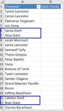
We’ll use the FIND function in order to identify any characters with ‘Stark’ in their name.
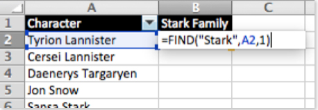
Pretty straight forward, I think. Here is the result!
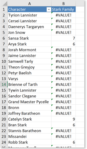
There are tons of #Value! errors (and my eyes are burning), but there are also some numbers. These numbers basically indicate which character the word “Stark” begins in the referenced cell. For cell A20 (Catelyn Stark), the word “Stark” begins on the 9th character in the cell.
Useless, right? For an excel noobie, but not you. You can nest the Find function with other functions and do some pretty cool things Lets extract the word “Stark” from the cell and display it in Column B:
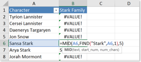
I nested the result of the FIND function (7) with the MID function and extracted the word “Stark” from the name in A6.
The best way to learn this is to get into Excel and start practicing with different examples that are more specific to you and your company.
Bonus functions: LEN & TRIM
LEN and TRIM are two functions that are also useful when dealing with texts. LEN returns the number of characters in a cell and TRIM removes any spaces before or after a string of alphanumeric characters.
You can NEST LEN with some of the other text functions to make your text extracting exercise even more dynamic and scalable.
If you use some of the functions we discussed earlier on a cell that has a space before of after the string of characters you’re analyzing, your functions won’t return what you’re expecting.
Here are both functions in action:

